One-dimensional Waves
Example from the PscFunctions package
Using PscFunctions routines it is possible to obtain a line of new exact formula solutions of some initial boundary value problems for the wave equation.
| > |
restart;
with(PscFunctions):
|
1.
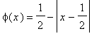
Finite string. Initial displacement is in the form of a triangle peak
.
Consider a finite string having length
L=1
. The string is fixed at both ends and have a zero initial velocity. The wave constant is
a=1
.
Execute odd periodic extension of the function
 (initial displacement) to entire axis with the help of
FPeriodic
routine of the package
(initial displacement) to entire axis with the help of
FPeriodic
routine of the package
| > |
f:=x->1/2-abs(x-1/2):
F:=FPeriodic(f,0..1,style='odd'):
F(x);
plot(F(x),x=-2..3,thickness=2);
|
![[Maple Plot]](DemoImages/OneDimensionalWave3.gif)
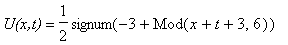
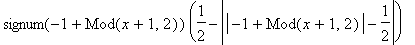
Function
Mod(x, y)
used in the previous formulas
gives the remainder on division of the first argument by the second.
Create a solution
u(x,t)
of the problem with usage of the d'Alembert formula taking into account that the initial velocity of the points of the string is equal to 0. Then we represent this solution
as an excited mode of the form
F(x-t)
moving toward the positive values of the
x-
axis with the velocity
a=1
and as another excited mode of the form
F(x+t)
moving with the same velocity in the opposite direction.
| > |
u:=(x,t)->(F(x+t)+F(x-t))/2:
plots[animate]( plot, [[u(x,t),F(x+t)/2,F(x-t)/2],x=-1..2,thickness=[3,2,2],color=[RED,BLUE,NAVY]], t=0..1.95, frames=40 );
print('u(x,t)'=u(x,t));
|
![[Maple Plot]](DemoImages/OneDimensionalWave4.gif)


2.
Finite string. Initial displacement is in the form of a narrow trapezium
.
Consider a finite string having length
L=
1. The string is fixed at both ends and have a zero initial velocity. The wave constant is
a=1
.
| > |
f:=FPolyline([[1/2,0],[3/5,1],[7/10,1],[4/5,0]]):
F:=FPeriodic(f,0..1,style='odd'):
u:=(x,t)->(F(x+t)+F(x-t))/2:
plots[animate]( plot, [u(x,t),x=0..1,thickness=2], t=0..1.95,frames=40 );
`U(x,t)`=u(x,t);
|
![[Maple Plot]](DemoImages/OneDimensionalWave7.gif)


3.
Finite string. Initial displacement is in the form of parabola that is oblique to the left
.
Consider a finite string having length
L=
1. The string is fixed at both ends and have a zero initial velocity.
| > |
f:=x->2*sqrt(x)*(1-x):
F:=FPeriodic(f,0..1,style='odd'):
u:=(x,t)->(F(x+t)+F(x-t))/2:
plots[animate]( plot, [u(x,t),x=0..1,thickness=2], t=0..1.95 ,frames=40);
`U(x,t)`=u(x,t);
|
![[Maple Plot]](DemoImages/OneDimensionalWave12.gif)


4.
Finite string. Initial displacement is in the form of the oblique triangle
.
Consider a finite string having length
L=
3. The string is fixed at both ends and have a zero initial velocity. .
| > |
f:=FPolyline([[0,0],[2,3],[3,0]]):
F:=FPeriodic(f,0..3,style='odd'):
u:=(x,t)->(F(x+t)+F(x-t))/2:
plots[animate]( plot, [u(x,t),x=0..3,thickness=2],t=0..5.9,frames=60 );
`U(x,t)`=u(x,t);
|
![[Maple Plot]](DemoImages/OneDimensionalWave15.gif)